Quick Start
Analyzing taxi traffic in New York
This example is based on the public dataset that can be found here .
It is a thirty million lines dataset with detailed taxi trips data for one year.
A subset (one month of data) is installed with the application package. It is available in the "Demo Files" folder.
Tutorial Overview
In this tutorial, we will build a workflow to clean and prepare raw data, followed by an analysis of traffic patterns. The focus will be on identifying trends by day of the week and categorizing trips based on their duration.
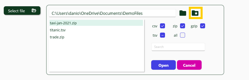
First step: preview and load data
When you select the file to load an instant preview of data will be available.

Data Preview and Type Inference
The preview displays the first 10,000 lines of the file. During this stage, heuristic rules are applied to infer the most appropriate data type and format for each column. For date fields, the system attempts to detect the format and distinguish between day/month and month/day ordering; in this case, it correctly identifies the American format (month before day). For numeric fields, it determines whether values are integers or floating-point numbers, and identifies the presence and style of thousands and decimal separators.
Manual Adjustment of Column Types
While data types and formats are generally inferred accurately during preview, manual configuration may be necessary in specific cases. For instance, a column containing only integers in the first 10,000 lines may later include floating-point values in the full dataset. Some patterns may also be misinterpreted due to limited preview data. A common example is the representation of monthly periods as values like 2022.01, which may be inferred as floating-point numbers. To enable operations such as extracting year and month components, it is recommended to explicitly set the column type to “string”.
Column Selection and Renaming
It may be necessary to exclude certain columns from processing and assign more descriptive names to others. In this example, the column “VendorId” is ignored, and the remaining columns are renamed for clarity. Additionally, the float precision is set to two decimal places.
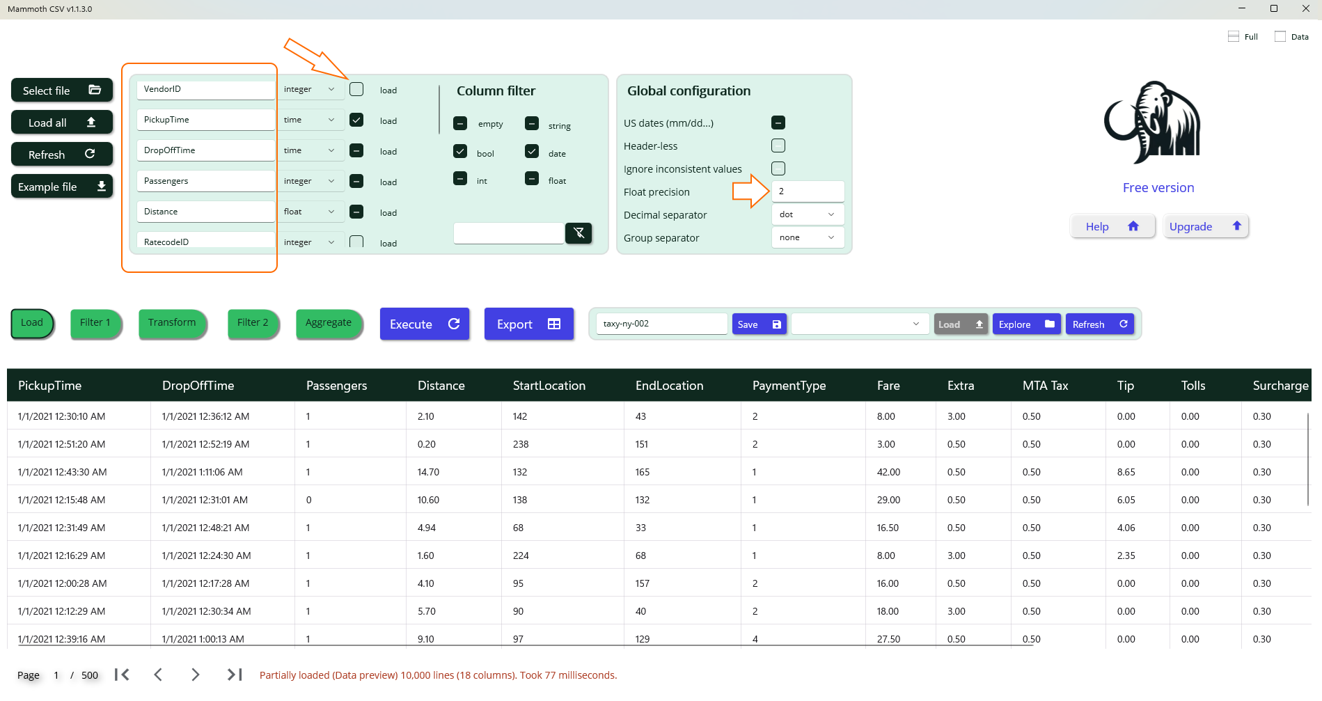
Once the layout is finalized, selecting the Load All button initiates loading of the entire dataset into memory. For a file containing 30 million rows and 18 columns, approximately 5 GB of memory is required.
Data Filtering Step
This step enables you to either isolate a specific subset of data or perform a cleanup operation on the entire dataset. Filtering is achieved through a sequence of basic logical conditions applied to column values. Each condition is defined by the following components:
- Column: The target column to evaluate.
- Operator: The logical comparison to apply (e.g., =, ≠, ≤, is empty, is not empty).
- Value(s): One or more values used for comparison (if applicable).
Operator Behavior
- = The condition passes if any of the specified values match.
- ≠ The condition fails if any of the specified values match.
- is empty and is not empty: These operators do not require any values.
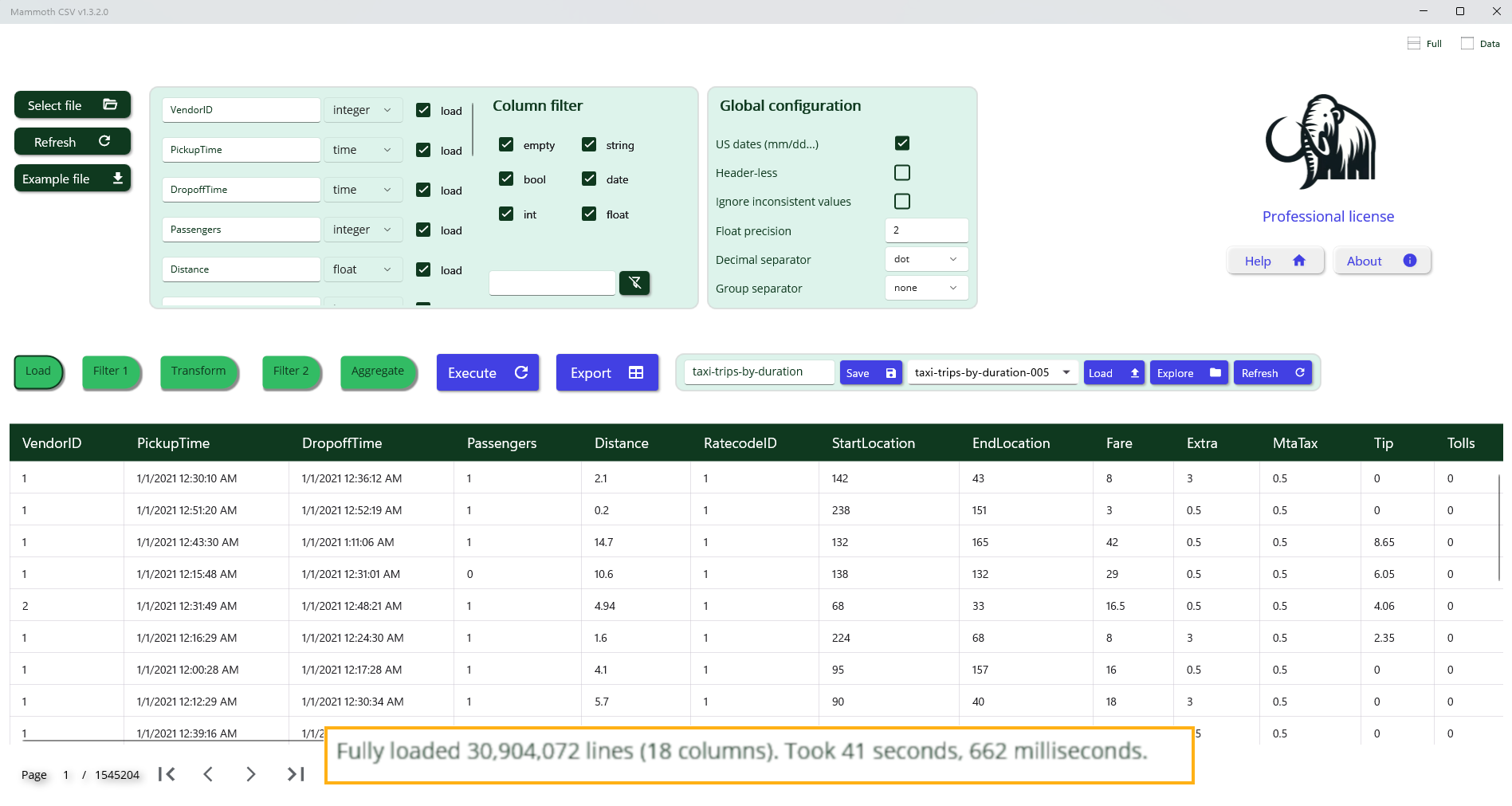
Example: Data cleanup filter
To remove invalid entries, apply a filter that excludes rows where PassengerCount or Distance are missing or contain invalid values.
Enriching Data with Computed Columns
This step allows you to define new columns derived from existing ones using a flexible formula language.
A comprehensive overview of available functions and operators is provided in the following section.
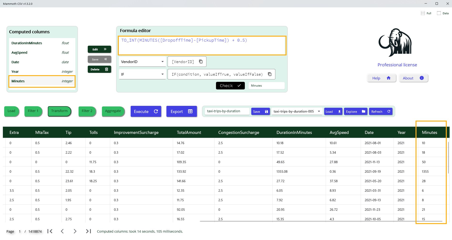
Example: Trip Duration in Minutes
To compute the trip duration in minutes and prepare it for use as an aggregation axis, we apply the following formula:
TO_INT(MINUTES([DropoffTime] - [PickupTime]) + 0.5)
Formula Breakdown
- Column reference: Use [ColumnName] to access the value of a specific column.
- Duration calculation: Subtracting [PickupTime] from [DropoffTime] yields a time interval.
- Unit conversion: The MINUTES() function converts the interval into minutes, resulting in a floating-point value.
- Rounding: Adding 0.5 before applying TO_INT() ensures standard rounding to the nearest integer.
- Integer conversion: The TO_INT() function truncates the floating-point result to the closest lower integer.
This computed column can then be used for grouping, aggregation, or further analysis.
Second-Level Filtering
An additional filtering layer is available via the Filter 2 tab. This step allows you to refine the initial filter by leveraging computed columns generated during the Transform phase.
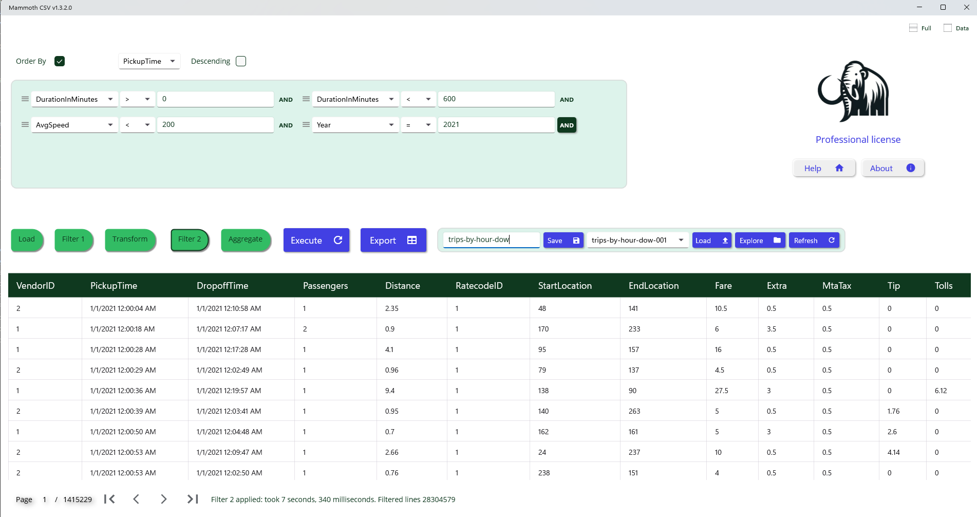
Use Case: Detecting Inconsistent Records
Computed columns can help identify and exclude rows with anomalous or illogical data patterns, such as:
- Drop-off time earlier than pickup time
- Unusually large trip distance with very short duration
- Suspicious or outlier trip durations
By applying logical conditions to these computed columns, you can effectively filter out invalid or inconsistent entries, improving overall data quality.
Pivot Table Computation – Multi-Axis Aggregation
Pivot tables enable structured data aggregation based on a defined set of axes and measures.
Axes
An axis is a column used to group data by its distinct values. Only columns with discrete value types can serve as axes, as equality must be well-defined. Continuous types (e.g., floating-point numbers or timestamps) are not suitable for axis-based grouping. Valid axis types include:
- Date columns (not raw timestamps)
- Integer values (not floating-point)
- Strings
- Boolean values
Measures
A measure is an aggregation function applied to a column, producing a summary value for each axis value (or combination of axis values).
Aggregation functions operate on:
- Numeric columns (integers and floating-point)
- Boolean columns
Most aggregation functions require a target column, except for Count, which simply returns the number of rows per axis group.
Supported aggregation functions:
Numerical:
- Count
- CountDistinct(column)
- Sum(column)
- Avg(column)
- Min(column)
- Max(column)
Boolean:
- All(column) – returns true if all values are true
- Any(column) – returns true if any value is true
This structure allows flexible multi-dimensional analysis across various data types
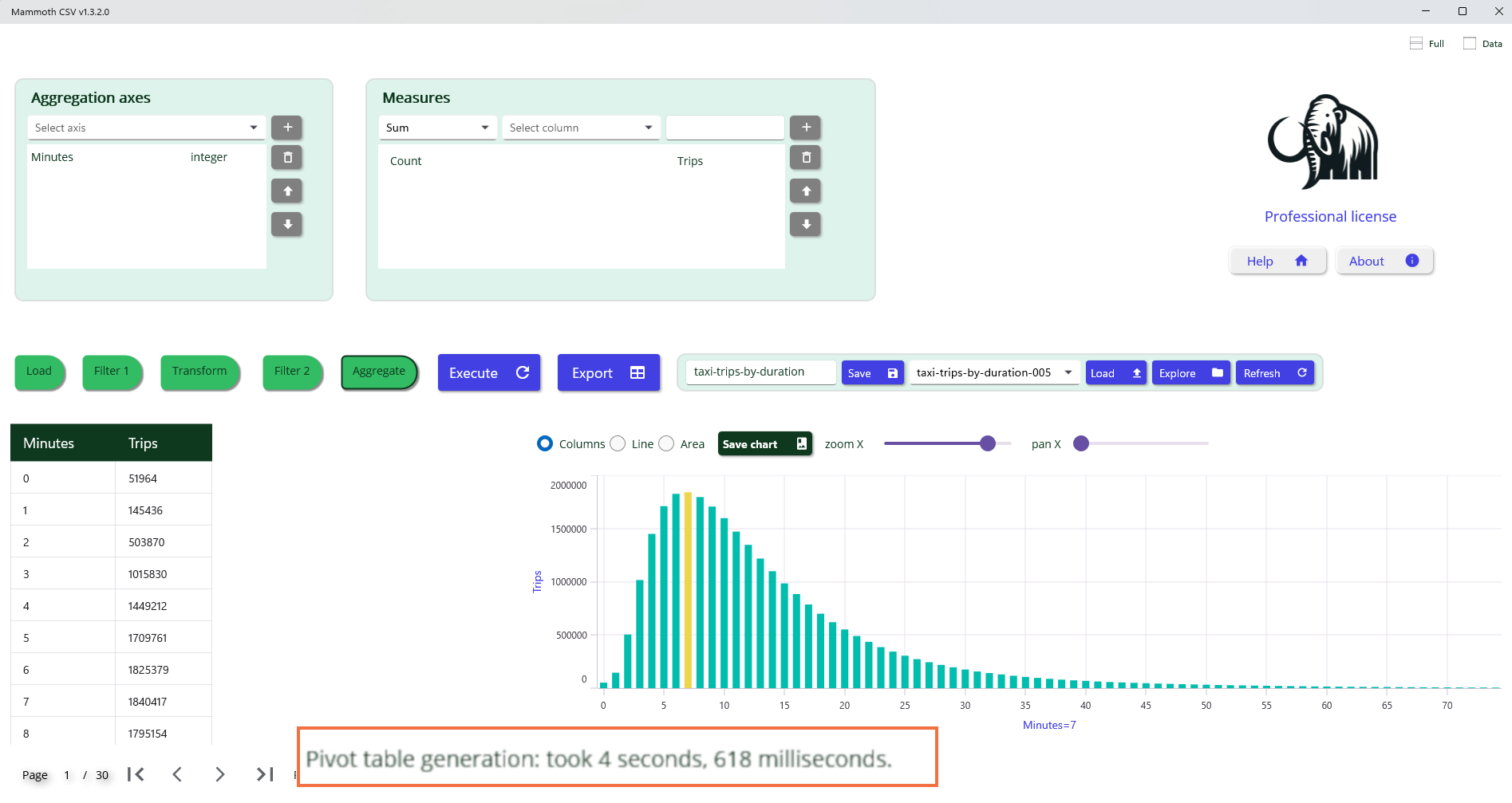
Insight from Visual Analysis
The image above reveals a key insight: most taxi trips in New York City have a duration of approximately seven minutes. This observation was derived from a dataset containing over 30 million records, processed and visualized without writing any code. The platform's built-in aggregation and filtering capabilities enabled rapid exploration and discovery of meaningful patterns. Such visual summaries are especially valuable for identifying dominant behaviors and guiding further analysis or operational decisions.